1. Description
Course STAT467 Multivariate Analysis
Semester Fall 2017
Content Multivariate Normal Distribution and Its Properties part:1*
Notebook Language R
*Notes are mostly from Applied Multivariate Statistical Analysis (Johnson et al.) and Applied Multivariate Statistical Analysis (Härdle et al.)
2. Probability Density Function of p-dimentional Normal Distribution
$$ X \sim N_p(\mu,\Sigma) $$$$f(x;\mu,\Sigma) = \frac{1}{2\pi^{(p/2)} |\Sigma|^{1/2}}e^{{-0.5(x-\mu)'\Sigma^{-1}(x-\mu)}}$$3. Probability Density Function of 2-dimentional (bivariate) Normal Distribution
we know;
$$ \sigma_{12} = \sigma_{21} = \rho_{12}\sqrt{\sigma_{22}\sigma_{11}} \tag{3} $$so;
$$ \Sigma^{-1} = \frac{1}{(1-\rho_{12})^2 \sigma_{11} \sigma_{22} } \left[ {\begin{array}{cc} \sigma_{22} & -\rho_{12}\sqrt{\sigma_{22}\sigma_{11}} \\ -\rho_{12}\sqrt{\sigma_{22}\sigma_{11}} & \sigma_{11} \\ \end{array} } \right] \tag{4} $$Rewrite the formula like:
$$ (x-\mu)'\Sigma^{-1}(x-\mu) = \frac{1}{(1-\rho_{12})^2 \sigma_{11} \sigma_{22} } \left[ {\begin{array}{cc} x_1-\mu_1 & x_2-\mu_2 \\ \end{array} } \right] \left[ {\begin{array}{cc} \sigma_{22} & -\rho_{12}\sqrt{\sigma_{22}\sigma_{11}} \\ -\rho_{12}\sqrt{\sigma_{22}\sigma_{11}} & \sigma_{11} \\ \end{array} } \right] \left[ {\begin{array}{c} x_1-\mu_1 \\ x_2-\mu_2 \\ \end{array} } \right] $$$$ (x-\mu)'\Sigma^{-1}(x-\mu) = \frac{(x_1-\mu_1)^2 \sigma_{22} + (x_2-\mu_2)^2 \sigma_{11} -2 \rho_{12} \sqrt{\sigma_{11}\sigma_{22}}(x_1-\mu_1)(x_2-\mu_2)}{(1-\rho_{12})^2 \sigma_{11} \sigma_{22}}$$Hence;
$$f(x;\mu,\Sigma) = \frac{1}{2\pi \sqrt{(1-\rho_{12})^2 \sigma_{11} \sigma_{22}}}e^{-0.5h(x;\mu,\Sigma)}$$4. R Function for p-dimentional Normal Distribution
4.1 Writing the density function
Let's partition above pdf into two pieces;
$$ h(x;\mu,\Sigma)=(x-\mu)'\Sigma^{-1}(x-\mu) $$$$ g(\Sigma) = 2\pi^{(p/2)} |\Sigma|^{1/2} $$Hence;
$$ f(x;\mu,\Sigma) = \frac{1}{g(\Sigma)}e^{-0.5h(x,\mu)} $$MultiNorm = function(x, M, S){
p = length(x) #number of observations
x = matrix(x, p, 1) #random variable vector
M = matrix(M, p, 1) #mean vector
h = t(x-M)%*%solve(S)%*%(x-M) #matrix multiplication that we defined earlier
g = ((2*pi)^(p/2)) * sqrt(det(S)) #normalizing constant
f = (1/g)*exp(-0.5*h) #density result
return(f)
}
4.2 Data Generation
Lets generate some M and S to test our function. This is NOT MVN distribution generator. I will just generate parameters of MVN distribution. (This section is more like a bonus section, if you like, you can continue with section 5)
p = 4
M = runif(p) #p means from 0-1 interval
V = runif(p, 1, 4) #p variances from 1-4 interval
I will not generate their Variance-Covariance matrix first. Instead, i will generate their correlation matrix and then find its Variance-Covariance matrix by using Variance and Correlation Matrix. In this way, i will have more control over linear dependency of variables.
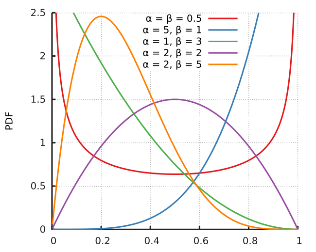
To generate its correlation matrix, i will use Beta distribution. Because it's interval is between 0 and 1. In addition, its shape quite flexible w.r.t. its parameters. If you want strong/weak correlation, you can generate them from a beta where a>b/b>a. Let's clearify it with an example;
set.seed(108)

print("from Beta(5, 1.5):")
print(rbeta(5, shape1 = 5,shape2 =1.5)) #right skewed (we could generate strong correlation)

print("from(Beta(1, 5):")
print(rbeta(5, shape1 = 1,shape2 =5)) #left skewed (we could generate weak correlation)
set.seed(108)

a = 1.5; b = 8 #we want a rather weaker correlation

P = diag(0.5, p, p) #diagonal of Correlation matrix = 1, because Cor(x, x) = 1

for(i in 1:(p-1)) for(j in (i+1):p) P[i, j] = rbeta(1, a, b) # I obtained an upper triangular matrix

P = P + t(P) # i added P with transpose of it. Because of symetric property of Correlation matrix

print(round(P, 2))
S = diag(V^(1/2)) %*% P %*% diag(V^(1/2))
print(round(S, 2))
Let's put it all together and create a parameter creation function for a Multivariate Normal distirbution.
p = (integer, scaler) number of variables
M_interval = (integer, size 2 vector) interval of mean
V_interval = (integer, size 2 vector) interval of variance
correlation = (charachter, scaler) Correlation magnitude of variables. It could be one of them: none, weak, modarate, strong
MVN_prm_genarator = function(p, M_interval, V_interval, correlation = "weak", myseed = 1){

    set.seed(myseed)

    M = runif(p, M_interval[1], M_interval[2])
    V = runif(p, V_interval[1], V_interval[2])

    if(correlation == "none"){
        S = diag(V) #if no correlation Var-Cov matrix is exactly equal to diagonal variance matrix
    }else{
        if(correlation == "weak"){
            a = 1.5; b = 8
        }else if(correlation == "moderate"){
            a = 2; b = 2
        }else{
            a = 5; b = 1
        }

        P = diag(0.5, p, p) #diagonal of Correlation matrix = 1, because Cor(x, x) = 1 (we will add it to 1)

        for(i in 1:(p-1)) for(j in (i+1):p) P[i, j] = rbeta(1, a, b) # I obtained an upper triangular matrix

        P = P + t(P) # i added P with transpose of it. Because of symetric property of Correlation matrix

        S = diag(V^(1/2)) %*% P %*% diag(V^(1/2))
    }

    return(list(M = M, S = S))
}
Hooray, we created our own parameter generation function for MVN distribution. With this function we could easily generate MVN's that have differenent characteristics.
MVN_prm_genarator(p = 10, M_interval = c(1, 4), V_interval = c(1, 10), correlation = "modarate")
MVN_prm_genarator(p = 3, M_interval = c(-2, 2), V_interval = c(1, 6), correlation = "none")
5. Plot p-dimentional Normal Distribution
library(plot3D)
library(plotly)
plot_mvn = function(MS, x1_interval, x2_interval){

    x1 = seq(x1_interval[1], x1_interval[2], length = 100)
    x2 = seq(x2_interval[1], x2_interval[2], length = 100)
    Mu = mesh(x1, x2)

    x = Mu$x
    y = Mu$y

    z = matrix(0, 100, 100)
    for(i in 1:100){
      for(j in 1:100){
        z[i, j] = MultiNorm(x = matrix(c(x[i, j], y[i, j]), 2, 1), M = MS$M, S = MS$S)
      }
    }

    df = list(x1 = x1, x2 = x2, z=z)

    plot_ly(x = df$x1, y = df$x2, z = df$z) %>% add_surface()
}
We are going to compare correlation effect into plot, with 4 different bivariate normal distributions all distirbuted with same mean and variances. But their correlations differ.
none = MVN_prm_genarator(p = 2, M_interval = c(0, 0), V_interval = c(10, 10), correlation = "none")
weak = MVN_prm_genarator(p = 2, M_interval = c(0, 0), V_interval = c(10, 10), correlation = "weak")
moderate = MVN_prm_genarator(p = 2, M_interval = c(0, 0), V_interval = c(10, 10), correlation = "moderate")
strong = MVN_prm_genarator(p = 2, M_interval = c(0, 0), V_interval = c(10, 10), correlation = "strong")
Let's print their Variance-Covariance matrices:
print("No covariance:")
print(none$S)

print("Weak covariance:")
print(weak$S)

print("Moderate covariance:")
print(moderate$S)

print("Strong covariance:")
print(strong$S)
x1_interval = c(-12, 12)
x2_interval = c(-12, 12)
print("No covariance:")
plot_mvn(none, x1_interval, x2_interval)
print("Weak covariance:")
plot_mvn(weak, x1_interval, x2_interval)
print("Moderate covariance:")
plot_mvn(moderate, x1_interval, x2_interval)
print("Strong covariance:")
plot_mvn(strong, x1_interval, x2_interval)
When two variables have equal mean and variances. The shape seems like a cone. But when covariance increase, shape of x-y plane became more elliptic. The reason behind this quite obvious. When X1 and X2 are positively correlated. They accumulate around a line that has positive slope in x1-x2 space. And negative slope line when correlation is negative.